“Portolan Numbers”
Before the mathematics governing cartographic projection was put to use, the most accurate maps of the middle ages were the portolan charts. This type of map was characterized by a “windrose network” of crisscrossing lines representing headings in the 16 directions from various points. These networks exhibit many beautiful and intricate patterns, and suggest a number of deep questions about mathematical objects like roots of unity, Chebyshev polynomials, and trigonometric diophantine equations.
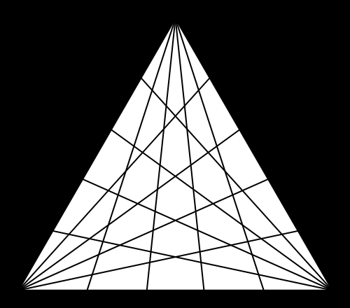
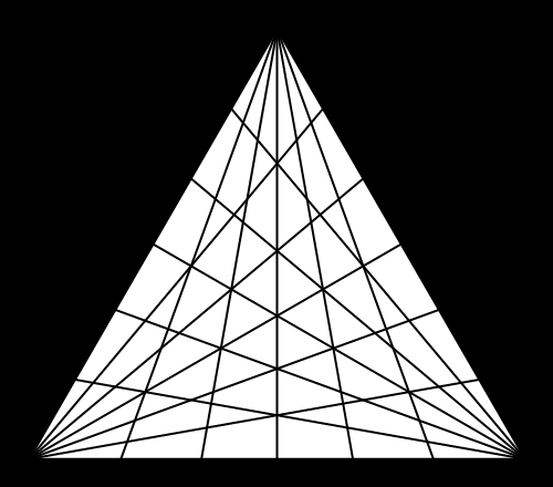
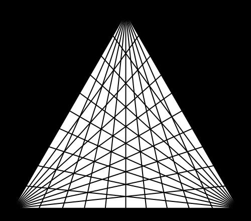
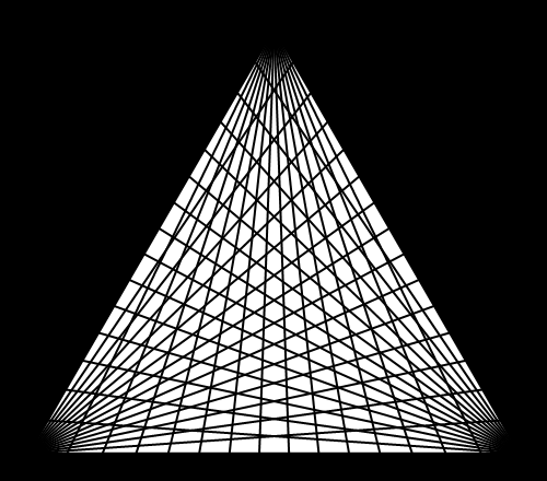
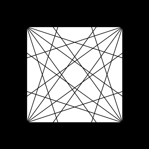
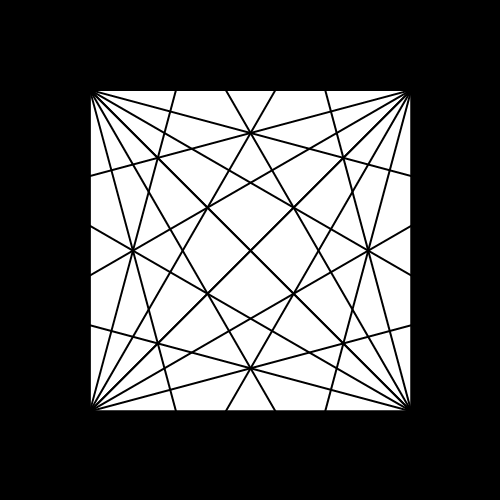
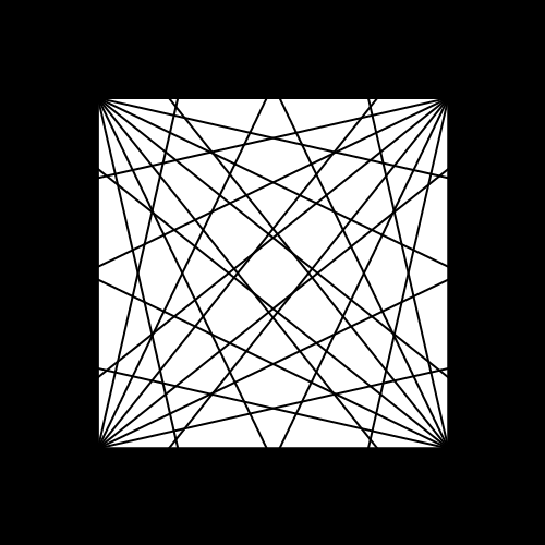
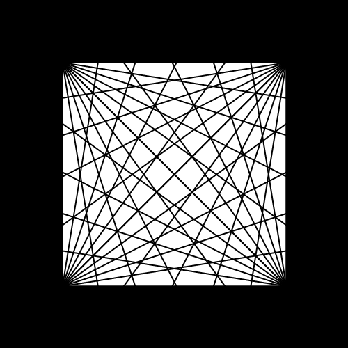
The theme of my investigation is the calculation of what I call “portolan numbers”: the number of regions you get when you draw lines out of each corner of a regular polygon to evenly divide the angles (splitting in two is bisecting, three is trisecting, …, n-secting). The real difficulty is finding out when more than two lines concur at a point: when this happens, naïve ways of counting fail. The real object of interest here, then, is not the number of regions, but the structure of the intersections. This structure can be linked to the divisibility properties of the integers and so is naturally addressed in the context of a field called algebraic number theory.
Chances are, though, you’re here to look at pretty pictures, not learn about algebraic number theory. Have at it, then:
-
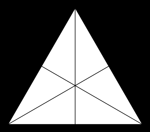
- P(3,2) = 6
-

- P(3,3) = 19
-

- P(3,4) = 30
-
- P(3,5) = 61
-
- P(3,6) = 78
-
- P(3,10) = 234
-
- P(3,15) = 631
-
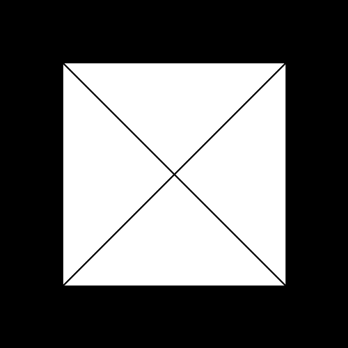
- P(4,2) = 4
-
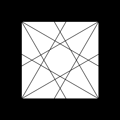
- P(4,3) = 29
-
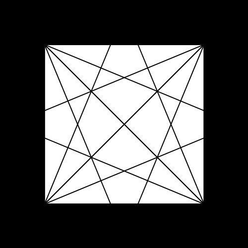
- P(4,4) = 32
-
- P(4,5) = 93
-
- P(4,6) = 84
-
-
P(4,7) = 189
Note the apparent 3-concurrences e.g. x=~1/3, y=~1/6. These are actually near-misses — there are tiny little regions in the middle of them.
-
- P(4,10) = 316
If you want to know more about the subject, see my entry at the Online Encyclopedia of Integer Sequences. I have some more notes there about the mathematics behind the n=3 case.
Subdividing Triangles through their Centers
From my interactive Wolfram Demonstration:
Associated with every triangle are a number of special points called “triangle centers.” Some of the best known of these include the centroid, incenter, and circumcenter; many more have been named and studied. Not all triangle centers, in fact, fall in the interior of a given triangle, but some always do. We can draw segments from the vertices to one of these interior triangle centers to subdivide the triangle into three new ones. Iterating this process can produce some beautiful figures. This Demonstration shows the centers of all the subtriangles up to the \[n\]th iteration.
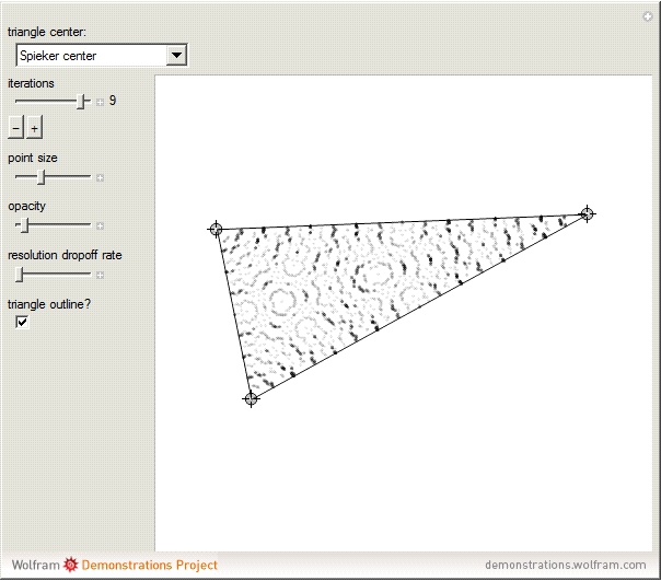
Subdividing through the Spieker center
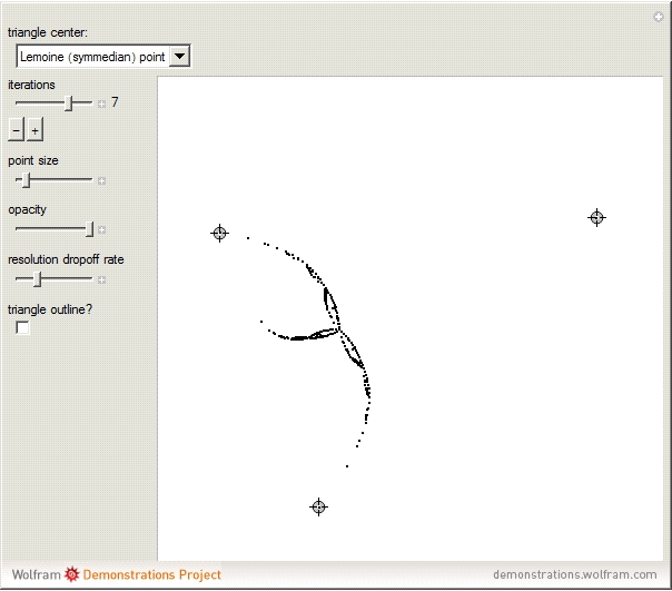
Subdividing through the Lemoine point
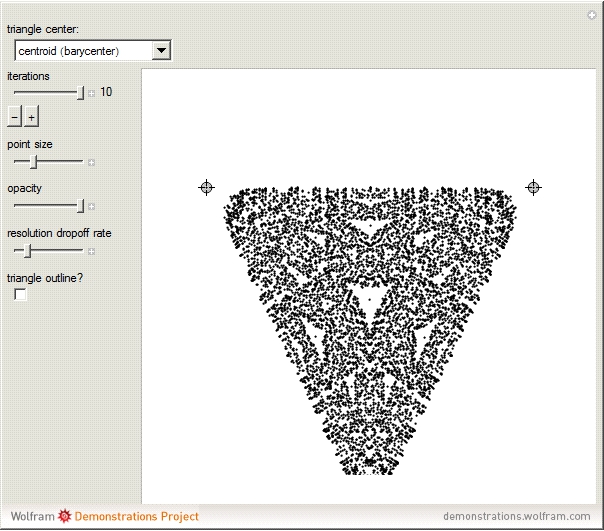
Subdividing through the centroid
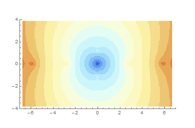
Continued Fraction Convergence Plots
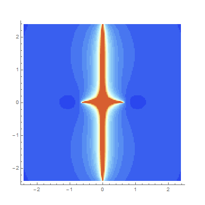
It’s pretty hard in general to determine if a generalized complex continued fraction, e.g.
$$c_0+id_0+\cfrac{a_1+ib_1}{c_1+id_1+\cfrac{a_2+ib_2}{c_2+id_2+\dots}}$$
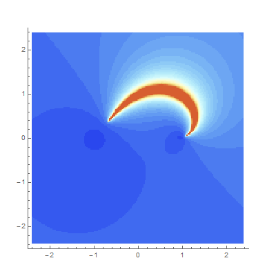
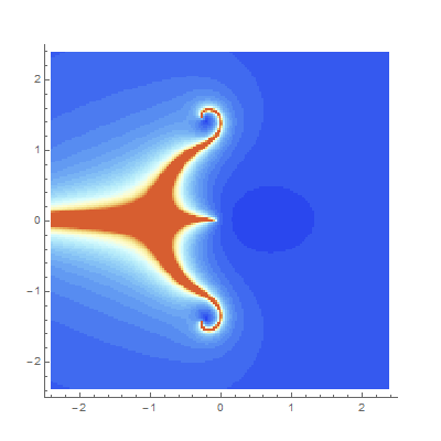
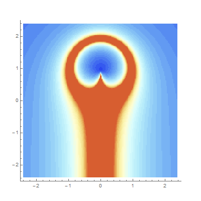
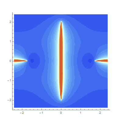
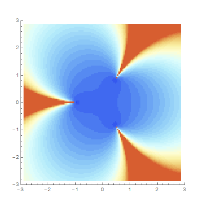
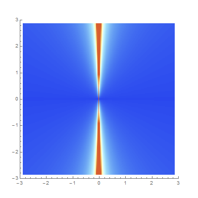
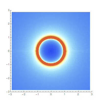
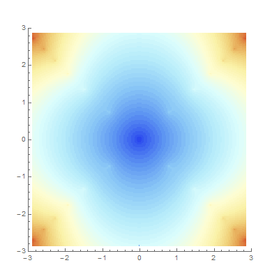
converges. But convergence plots à la Mandelbrot can give us some intuition, and furthermore they tend to be quite pretty. These plots each show how quickly continued fractions derived as functions of a complex parameter \[z\] converge. We try to map
$$z \mapsto {\large K}_{z=0}^\infty \frac{f(z)}{g(z)},$$
but sometime this transformation yields an actual number (the CF converges) and sometimes it doesn’t. Each point is colored according to how many iterations it takes for the difference between iterates to shrink below a certain tolerance. The redder a point is, here, the longer it takes.
-
- K z^2-1 / z^2+1
-
- K z^2-1 / z-(1+1)
-
- K z^3+2z-1 / z^2+2.1
-
- K iz+1 / .5z-i
-
- K cos z / sin z
-
- K z^3 / 1
If we let \[T_z(\zeta) = \frac{f(z)}{g(z)+\zeta}\], then these plots help us investigate the orbits of various \[T_z\]s on an arbitrary \[\zeta\] (exercise: why is zeta arbitrary? Is it ever not?). A slightly more complicated, but far more general, research subject varies \[T_{z,j}\] with \[j\], which is an integer indexing the depth of our fraction. Then we can look at how-long-til-convergence plots of \[z \mapsto {\large K}_{z=0}^\infty \frac{f_j(z)}{g_j(z)}\] — sequences of \[f\]s and \[g\]s (equivalently, \[T\]s). This allows us to look at well-known continued-fraction versions of common functions, as well as a few more exotic CFs.
-
- CF for atan[im(z)/re(z)]
-
- CF for log(1+z)
-
- z^2 / (1+ K (-1)^j*jz^2 / j )
-
- CF for tan(z)
Cesàro Curves
Plotting members of a one-complex-parameter family of fractal curves, obtained as the limit of a sequence of affine transformations on the complex plane.
-

- a = .2+.25i
-

- a = .9+.35i
-
- a = .58+.2i